
Lab 7: Timing Experiments
Lectures needed for this lab: Lecture 8 (Resizing and Circular Arrays) and Lecture 13 (Asymptotics I), or Chapter 8 and Chapter 12.
FAQ
Each assignment will have an FAQ linked at the top. You can also access it by adding “/faq” to the end of the URL. The FAQ for Lab 7 is located here.
Introduction
Different data structures perform differently in different situations. In this
lab, we’ll explore a couple of these situations, ending with the AList
class we discussed in lecture.
Goals and Outcomes
In this lab, you will solidify your understanding of asymptotic analysis:
By the end of this lab, you will…
- Understand that different data structures and algorithms have different time guarantees.
- Be able to empirically measure the runtime of a piece of code.
- Interpret timing experiments and reason about their implications.
Setup
Follow the Assignment Workflow Guide to get started with this assignment. This starter code is in the lab07 folder. NOTE as with previous labs you do not need to submit this assignment. Instead, you will get credit by completing a checkpoint with your TA during lab.
Timing Experiments
Overview
One way of determining the speed of a given program is to test it on a variety of inputs and measure the time it takes for each one. This is called a timing experiment, and we refer to this process as finding the efficiency of a program empirically.
This is a natural complement to what we’ve done in lecture, where we’ve discussed how we can theoretically model the runtime of a segment of code using big theta (and big O and big Omega) notation.
In this lab, you’ll analyze code by hand to predict the runtime behavior of different pieces of code, then you’ll run experiments to validate that model.
In this part of the lab, we will be working with the code in the timing
package.
TimingData
In a timing experiment, we are interested in seeing how the time of some operations scales with the size of the computation. The output of a timing experiment will be an instance of the following class:
public class TimingData {
    public static class Trial {
        private final int N;          // the size of the input
        private final int ops;        // how many operations were timed
        private final double seconds; // how long those operations took, in total
        public double usPerOp() { ... }  // average microseconds per operation
    }

    private final String name;
    private final List<Trial> trials;

    public void add(int N, int ops, double seconds) { ... }
    // Some utility methods for accessing data
}
A TimingData object records all timing information for a given experiment. Each
TimingData contains a List<Trial>. A Trial represents the runtime results
for a single N. For example, if you ran an experiment which called contains
on a list with N = 100, N = 1000, and N = 10000, you’d end up with a TimingData
object with three Trial objects in its list.
A Trial has three instance variables and a method:
N: The size of the data structure, or how many elements it contains.ops: The number of operations that were timed. For example, we might do many operations to take an average over.seconds: The total time required for allopsoperations, in seconds.usPerOp(): The average time per operation, in microseconds:seconds / ops, converted to microseconds. This is the number we will most often use. Hereusmeans microseconds.
For the running example above of an ArrayList timing experiment, we might run contains
10,000 times for each N to reduce the noiseness of our timing. That is, we’d create
a list with N = 100, then call contains 10,000 times on that, then N=1000, then call
contains 10,000 times on that, and so forth. This is similar to remeasuring the
length of an object with a tape measure multiple times.
Example: ArrayList Timing
As a first example, let’s time how the runtime for the contains operation of an ArrayList
changes as a function of the number of items in the ArrayList.
Open timing/Experiments.java and look at exampleListExperiment. The key components of the
test are below:
int ops = 10000;

for (int N = 1000; N <= 512000; N *= 2) {
    ArrayList<Integer> list = new ArrayList<>();
    for (int i = 0; i < N; i += 1) {
        list.add(i);
    }
    Random random = new Random(61);

    Stopwatch sw = new Stopwatch();
    for (int j = 0; j < ops; j += 1) {
        list.contains(random.nextInt(N));
    }
    td.add(N, ops, sw.elapsedTime());
}
- For each
Nfrom 1000 up to 512000, doubling each time, we build anArrayListholding the numbers0throughN - 1. ThisNis the size of the trial. - A single
containscall on a list of 1000 items takes about a microsecond, which is far less than our stopwatch can see: it only counts milliseconds. So each trial callscontains10,000 times, andopsis10000. The trial’susPerOp()then tells us the average cost of onecontains. - To time code, we use Princeton’s
Stopwatchclass. We construct aStopwatchjust before the code we want to time, and callstopwatch.elapsedTime()at the end to see how much time has passed in seconds. That is the trial’sseconds. - Notice that we build the list before we start the
Stopwatch. We’re measuring onlycontains, notadd.
If you run this code you’ll get something like:
           N     time (s)        # ops  microsec/op
------------------------------------------------------------
        1000         0.01        10000         0.70
        2000         0.00        10000         0.20
        4000         0.01        10000         0.50
        8000         0.01        10000         0.90
       16000         0.02        10000         1.90
       32000         0.04        10000         3.60
       64000         0.07        10000         6.90
      128000         0.14        10000        13.90
      256000         0.30        10000        30.30
      512000         0.58        10000        57.90
The first 3 columns are the Trial instance variables as described above. The
last column is the result of the usPerOp method, which provides the number of microseconds it took on average
to perform each operation. Here, an “operation” is a call to contains(). Note
that ops is always the same here, because we were timing the same number of
calls every time.
The times that you get on your computer may be very different from the table that’s written above. That’s okay, as long as the general trend is the same. In 61C, you will learn exactly why the same code may take vastly different amounts of time on different hardware. In 61B (and in most theory-based classes) we are only concerned with general trends, which hide parts of reality that are hard to account for. As we’ve seen in lecture, we can formalize this idea of the “general trend” by using big theta notation.
While we can do some things with numbers, it’s hard to really feel the “order of growth” in a text table. We can also use a graphing library to generate plots!
main also pops up a plot of the last column against N:
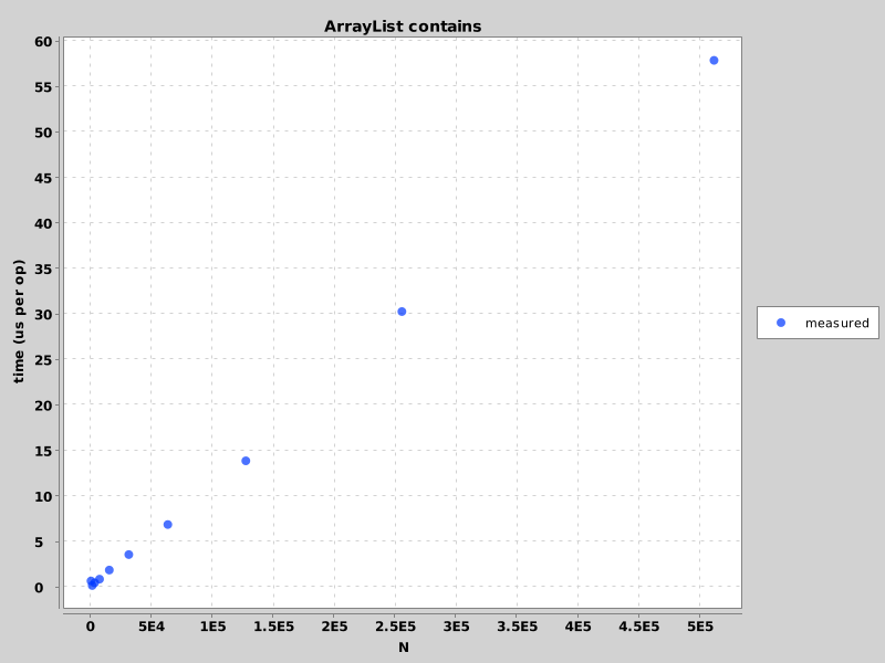
contains gets slower in direct proportion to N: double the list, double the
time. For example, observe that for N = 4,000 a lookup takes about 0.5 microseconds,
while for N = 512,000, a list 128 times bigger, it takes about 58 microseconds:
roughly 116 times longer.
This is because the contains method of an ArrayList has a Θ(N) runtime: it
checks the items one at a time, from the front, until it finds a match.
Example: Fibonacci
As another example, let’s look at timing a method that computes the N-th Fibonacci
number, very inefficiently. Open timing/FunctionsToBeTimed.java and look at
fib, then open timing/Experiments.java and look at exampleFibonacciExperiment.
The most interesting part is the for loop in the experiment:
int ops = 1;

for (int N = 25; N <= 40; N++) {
    Stopwatch sw = new Stopwatch();
    int fib = FunctionsToBeTimed.fib(N);
    td.add(N, ops, sw.elapsedTime());
}
- We compute the 25th through 40th Fibonacci numbers in the outer loop. Here
Nis the argument tofib. - Unlike
contains, one call tofib(N)is slow for theseN: a few milliseconds atN = 30and about a quarter of a second atN = 40. That is plenty for the stopwatch to measure on its own, so each trial times a single call andopsis1.
Timing Tables
Below, we show the table we got for Fibonacci when we ran the code.
           N     time (s)        # ops  microsec/op
------------------------------------------------------------
          25         0.00            1      1000.00
          26         0.00            1         0.00
          27         0.00            1      1000.00
          28         0.00            1      1000.00
          29         0.00            1      1000.00
          30         0.00            1      2000.00
          31         0.00            1      4000.00
          32         0.01            1      6000.00
          33         0.01            1      9000.00
          34         0.02            1     15000.00
          35         0.02            1     24000.00
          36         0.04            1     39000.00
          37         0.06            1     64000.00
          38         0.10            1    103000.00
          39         0.17            1    167000.00
          40         0.27            1    273000.00
The first 3 columns are the data we collected and described above. The last
column, as its header says, is the number of microseconds it took on average
to perform each operation. Here, an “operation” is a call to fib(N). Note
that ops is always the same here, because we were timing the same number of
calls every time.
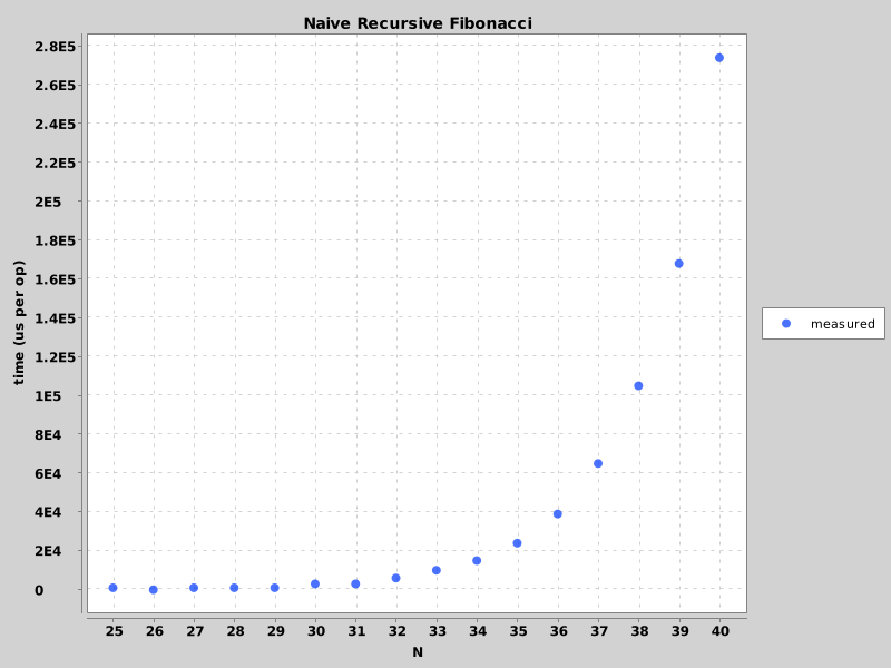
Here are some things to notice about the above table:
-
For 25, 27, 28, and 29, the time per
fib(N)call comes out exactly the same (one millisecond), and for 26 it comes out as zero, even though each of these calls is about 1.6 times slower than the one before it. For small inputs, timing results are not precise for two reasons:- The variance in runtime is high, for reasons beyond the scope of the course (and covered in CS 61C).
- The accuracy of our System clock (milliseconds) is insufficient to resolve the difference between runtimes for these calls.
This can also lead to strange situations, such as the runtime for 26 being smaller than the runtime for 25. Therefore, when we use empirical timing tests, we focus on the behavior for large
N– note that the differences are much larger, and easier to distinguish!
Fibonacci runtime Plot
Timing sp16fp9p1
Now it’s your turn to run a timing experiment from scratch. In FunctionsToBeTimed.java you’ll find the method sp16fp9p1. This method comes from the Spring 2016 final, and is problem 9,
part 1.
public static long sp16fp9p1(int N) {
    long sum = 0;
    for (int i = 0; i < N; i += 1) {
        for (int j = 1; j < N; j = j + 2) {
            sum += j;
        }
    }
    return sum;
}
Before doing an empirical test, talk with your partner/group: How do you think the runtime of sp16fp9p1 grows with N? Is it Θ(N)? Θ(N^2)? Something else?
Then measure it. Like the Fibonacci example it’s fine if ops is 1 because a single
call to sp16fp9p1(N) already does a lot of work.
Task: Implement timeSp16fp9p1 in Experiments.java. For N = 4000, 8000,
16000, 32000, 64000, and 128000, time one call to sp16fp9p1(N) and record the
trial with ops = 1. Then change main to run timeSp16fp9p1 and look at the plot.
Note: each sum += j is extremely fast, which is why N has to be so much
larger than in the Fibonacci example before the times are big enough to measure.
The small-N trials may well show 0.00 seconds. As always, focus on the trend
at large N. If the largest trial takes more than a couple of seconds on your
computer, stop at 64000 instead.
Empirical Fitting
Looking at the plot, you can probably tell the curve isn’t a straight line, but
is it N log N? N^2? Something else? Eyeballing a curve is unreliable, so
we’ve provided code that does the comparison for you. Fit.plotWithFit takes
a TimingData and a guess at the order of growth, finds the best-fitting curve
of that shape (the a * f(N) + b that comes closest to your data points), and
draws it over your timing plot. The legend shows the fitted curve and its
R^2, a measure of how well it fits: 1 is a perfect fit, and lower is worse.
For example, to see how well N^2 describes sp16fp9p1, change main to:
TimingData td = timeSp16fp9p1();
printTimingTable(td);
Fit.plotWithFit(td, Fit.Growth.N_SQUARED);
The available choices are Fit.Growth.CONSTANT, LOG_N, N, N_LOG_N,
N_SQUARED, N_CUBED, and TWO_TO_THE_N.
Task: Run plotWithFit on your sp16fp9p1 data with at least LOG_N, N,
N_LOG_N, and N_SQUARED. Which one fits best? Look at both the picture and
the R^2. Does the winner match what you expected from reading sp16fp9p1? Keep this
code handy, you’ll want to show it when you do the checkpoint.
More Functions to Time
Now do the same for three more functions from FunctionsToBeTimed.java. For
each one: predict its order of growth from the code, implement the timing
method in Experiments.java (one call per trial, ops = 1, over the given
range of N), look at the plot, then use Fit.plotWithFit to find the best
fit. Keep notes, you may be asked about any of them during your checkpoint.
sp16fp9p2
public static long sp16fp9p2(int N) {
    long sum = 0;
    for (int i = 0; i < N; i += 1) {
        for (int j = 1; j < N; j = j * 2) {
            sum += j;
        }
    }
    return sum;
}
Task: Implement timeSp16fp9p2 for N = 1,000,000 doubling up to
128,000,000. Which growth function fits best? Two of the candidates will fit
almost equally well, so here you’ll need to rely on your theoretical analysis
to differentiate them.
msf
public static long msf(int N) {
    if (N <= 1) {
        return 1;
    }
    long sum = 0;
    for (int i = 0; i < N; i += 1) {
        sum += i;
    }
    return sum + msf(N / 2) + msf(N / 2);
}
Task: Implement timeMsf for N = 1,000,000 doubling up to 64,000,000.
msf does N steps of work and then calls itself twice on half the size, etc.
Which growth function fits best? Think about how much work happens at each level of the recursion, and how many levels there are.
Note: The reason we learn to time strange functions like these is that they
exactly match the “shape” of real algorithms and data structures. For example,
in class, the weird function printParty very closely approximated the
runtime behavior of an ArrayList with resizing. What real algorithm does the msf
function behave like in terms of runtime?
sp16fp9p5
public static long sp16fp9p5(int N) {
    long sum = 0;
    for (long i = 1; i <= (long) N * N; i *= 2) {
        for (long j = 0; j < i; j += 1) {
            sum += j;
        }
    }
    return sum;
}
Task: Implement timeSp16fp9p5 for N = 1000 doubling up to 32000. Which
growth function fits best?
AList, Bad Resizing
As discussed in lecture, a multiplicative resizing strategy will result in fast add operations (good performance), while an additive resizing strategy will result in slow add operations (bad performance). In this part of the lab, we’ll put visuals to these statements!
In the timing package, we’ve provided the AList class created in lecture
with the bad resizing strategy below:
public void addLast(Item x) {
    if (size == items.length) {
        resize(size + 1);
    }

    items[size] = x;
    size = size + 1;
}
In this part of the lab, you’ll write code that tabulates the amount
of time needed to create a AList of various sizes using the addLast method
above.
Nshould take on the values of 1000, 2000, all the way to 128000, doubling each time.- You should time the entire time it takes to construct an
AListof sizeNfrom scratch. That is, you will need a newAListfor each value ofN, and you will have an inner for loop containing a call toaddLast. - We’re interested in the average time per
addLastcall, so the number of operations is the number ofaddLastcalls, orN.
Task: Implement
timeAListConstruction to perform a timing experiment with the aforementioned
specification. Make sure to replace the function call in main to be
timeAListConstruction! You may find it helpful to look at the code where we
timed ArrayList operations.
Note: If your computer is a little slow, you might want to stop at 64000 instead of 128000.
AList, Good Resizing
Task:
Modify the AList class so that the resize strategy is multiplicative
instead of additive and rerun timeAListConstruction.
Your AList objects should now be constructed nearly instantly, even for N =
128000, and each add operation should only take a fraction of a microsecond.
You might observe some strange spikes for “small” N – these are due to,
again, 61C material.
Optional: Try increasing the maximum N to larger values, e.g. 10 million. You
should see that the time per add operation remains constant.
Optional: Try experimenting with different resizing factors and see how the
runtimes change. For example, if you resize by a factor of 1.01, you should
still get constant time addLast operations! Note that to use a non-integer
factor you’ll need to convert to an integer. For example, you can use
Math.round().
public void addLast(Item x) {
    if (size == items.length) {
        resize((int) (size * 1.01));
    }

    items[size] = x;
    size = size + 1;
}