
Lab 11: Seam Carving
This is a lab about shortest paths, but from a different perspective. You’ll need Lecture 25 (Directed Acyclic Graphs), or Chapter 24 to fully understand what’s going on, though you can get by without. It also helps to remember shortest paths from Lecture 23 / Chapter 22.
Note: This lab is a bit different than others. In this lab, rather than reinforcing a specific core data structure or algorithm from lecture, we’ll instead explore how the idea of shortest paths on a graph can be used for the purpose of image resizing.
Here are the slides presented in lab for your reference.
FAQ
Each assignment will have an FAQ linked at the top. You can also access it by adding “/faq” to the end of the URL. The FAQ for Lab 11 is located here.
Introduction
Seam-carving is a content-aware image resizing technique where the image is reduced in size by one pixel of height (or width) at a time. That is rather than shrinking an image proportionally, it lets us cut shrink in only one dimension. It does this by repeatedly removing “seams”.
A vertical seam in an image is a path of pixels connected from the top to the bottom with one pixel in each row. (A horizontal seam is a path of pixels connected from the left to the right with one pixel in each column.) Below is the original 507-by-285 pixel image.
Further below we see the result after removing 150 vertical seams, resulting in a 30% narrower image while preserving the original width. Note that the image is not cropped, scaled, or distorted. Instead, the less important parts of the image have been removed, while the most interesting features of the image are preserved.


In this lab, you will create a data type that resizes a W-by-H image using the seam-carving technique, and then watch it work in your browser.
Goals and Outcomes
By the end of this lab, you will…
- Have implemented a shortest paths algorithm that finds the cheapest path through a grid, solving each row’s subproblems from the row above.
- Have seen that “shortest path in a DAG” and “fill in a table one row at a time” are the same idea.
- Have a seam carver that can shrink any photo you drop into it.
Setup
Follow the Assignment Workflow Guide to get started with this assignment. This starter code is in the lab11 folder. NOTE as with previous labs you do not need to submit this assignment. Instead, you will get credit by completing a checkoff with your TA during lab.
The three parts of the starter code you’ll care about are:
| File | What’s in it |
|---|---|
src/SeamCarver.java |
This is where you write code. |
src/SeamCarverVisualizer.java |
Run this to open the browser visualizer (described below). |
images/ |
Small test images, each with a .printseams.txt file giving its energies and seams. Also the surfing photo above. |
Notation. In this lab, pixel (x, y) refers to the pixel in column x and row y, with pixel (0, 0) at the upper left corner and pixel (W − 1, H − 1) at the bottom right corner, as shown below:
| (0, 0) | (1, 0) | (2, 0) |
| (0, 1) | (1, 1) | (2, 1) |
| (0, 2) | (1, 2) | (2, 2) |
| (0, 3) | (1, 3) | (2, 3) |
Warning: this is the opposite of the standard mathematical notation used in linear algebra where (i, j) refers to row i and column j and with Cartesian coordinates where (0, 0) is at the lower left corner.
Colors are given by a java.awt.Color object, where each color is a mix of a
red, green, and blue value (as shown in the next section).
Part 1: Pixel Energy (Intuitively)
The first step of seam carving is to calculate the energy of each pixel, which is a measure of the importance of each pixel: the higher the energy, the less likely that the pixel will be included as part of a seam.
The intuition is that a smooth part of an image is “low energy”, whereas a part of the image where the image is changing is “high energy”. In seam carving, we’ll ultimately be throwing away the low energy pixels.
Here is a photo of a recycling bin (with a surprise inside). Click the button to see the energy of every pixel, drawn as a grayscale image where brighter means higher energy.
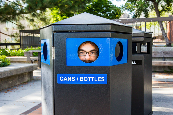
Notice where the energy is low: the flat sides of the trash can, the pavement, and the patches of sky. These are pixels you could remove without anyone noticing. Notice where it’s high: the lettering, the edges of the bin, the leaves, and the face. Those are the pixels we want to keep because removing them would be more noticeable.
If we were able to find a seam that only ever steps through low energy pixels, its removal would be almost invisible. By repeating this process we can downscale an image.
Part 2: Computing Pixel Energy
This section isn’t strictly necessary, but we recommend it so you can understand what’s really going on with the algorithm. Your choice whether to read!
We use the dual gradient energy function. In pseudocode, we compute as follows: Given a pixel P:
- Consider that P’s left neighbor L and right neighbor R.
- Compute $(L.red - R.red)^2 + (L.green - R.green)^2 + (L.blue - R.blue)^2$. This is the x-energy.
- Consider P’s up neighbor U and down neighbor D.
- Compute $(U.red - D.red)^2 + (U.green - D.green)^2 + (U.blue - D.blue)^2$. This is the y-energy.
- The total energy is the x-energy plus the y-energy.
We define the energy of pixels at the border by wrapping around, i.e. if we go off the image, we replace the non-existent pixel with the pixel from the opposite edge.
As an example, consider the 3-by-4 image with RGB values (each component is an integer between 0 and 255) as shown in the table below.
| (255, 101, 51) | (255, 101, 153) | (255, 101, 255) |
| (255, 153, 51) | (255, 153, 153) | (255, 153, 255) |
| (255, 203, 51) | (255, 204, 153) | (255, 205, 255) |
| (255, 255, 51) | (255, 255, 153) | (255, 255, 255) |
Tip: hover your mouse over (or tap) any of the underlined squared terms in the example below to highlight the two values in the table that it comes from.
We calculate the energy of pixel P = (1, 2), the shimmering cell above, in detail. Its left neighbor is L = (0, 2) = (255, 203, 51) and its right neighbor is R = (2, 2) = (255, 205, 255), so
x-energy = (255 − 255)2 + (203 − 205)2 + (51 − 255)2 = 0 + 4 + 41616 = 41620.
Its up neighbor is U = (1, 1) = (255, 153, 153) and its down neighbor is D = (1, 3) = (255, 255, 153), so
y-energy = (255 − 255)2 + (153 − 255)2 + (153 − 153)2 = 0 + 10404 + 0 = 10404.
Thus, the energy of pixel (1, 2) is $41620 + 10404 = 52024$.
Second Example: The energy of pixel (1, 1) is $204^2 + 103^2 = 52225$. (Its left and right neighbors differ only in blue, by 204, and its up and down neighbors differ only in green, by 103.)
Examples Summary: The energies for each pixel is given in the table below, where the shimmering entry is the one we calculated above.
| 20808.0 | 52020.0 | 20808.0 |
| 20808.0 | 52225.0 | 21220.0 |
| 20809.0 | 52024.0 | 20809.0 |
| 20808.0 | 52225.0 | 21220.0 |
Note that the energy of a pixel doesn’t depend on its color, but only on the colors of its neighbors.
Now test your understanding on a fresh pixel. Compute the x-energy, y-energy, and total energy of the center pixel below and type it in. The four neighbors you need are shown with their RGB values. The corners and the center pixel’s own color don’t matter.
energy(int x, int y) in SeamCarver is already written and does exactly
this computation for every pixel of the picture, with neighbors off the edge
wrapping around to the opposite side. The results are stored in a
double[][] energy table, indexed energy[x][y], that is recomputed whenever
the picture changes.
Part 3: The Visualizer
Run SeamCarverVisualizer. It starts a small web server and opens a page in
your browser (if nothing opens, go to the address it prints, which is
http://localhost:4567/). The page starts out showing the surfing photo from
the top of this page.
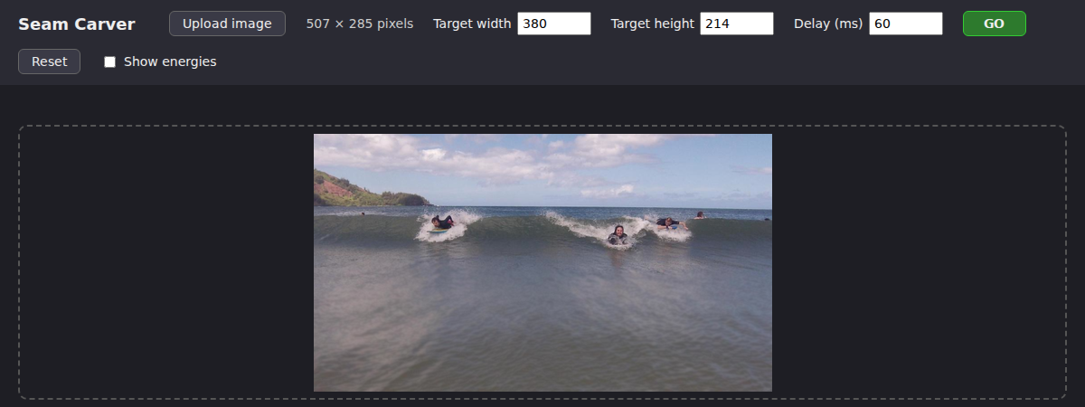
Load an image of your choosing: drag any photo onto the page, or click
Upload image and pick one of the photos from the images folder or one
of your own. If the photo is more than 500 pixels on a side, you’ll be asked
whether to use it at full scale (slow) or reduced scale (fast): pick
reduced. Then check Show energies and see if the energy image matches
your intuition about which parts of the picture are smooth.
Now uncheck Show energies, and look at the controls. Target width and Target height start out at 75% of the picture’s size. Click GO.
Nothing happens, except for a message that findVerticalSeam returned
null. The visualizer works by repeatedly asking your SeamCarver for a
seam, drawing it in red, and removing it, and the two methods that
findVerticalSeam relies on, computeM and findSeamFromM, are not written yet.
That’s your job!
Let’s now talk about the seam carving algorithm.
Part 4: Finding a Seam by Hand
Below is a tiny 10-by-10 picture, drawn as its energy: each square is a pixel, brighter means higher energy, and the number on each square is its energy.
A vertical seam is a path from the top row to the bottom row with exactly one pixel in each row, where each pixel is directly below, below-left, or below-right of the one above it.
The best seam is the one with the smallest total energy.
Build the minimum energy seam by clicking one pixel per row, starting at the top: first a pixel in the top row, then one of the three pixels below it, and so on. The running total of your seam is shown under the picture. To change your mind, click a pixel in an earlier row and continue from there. When you reach the bottom, click CHECK.
We observe that the greedy choice (here greedy means always take the cheapest next pixel) does not necessarily find the best seam.
One approach to finding the best path would be to treat this like a directed graph with a virtual top and virtual bottom node and run the Dijkstra’s that you impelemented in lab 10 (with modifications for handling a directed graph unlike an undirected graph as in lab 10).
However, this approach would be very slow because it would require the construction of an explicit Graph object with potentially millions of nodes and millions of edges. For example, the graph for the image above would look like shown below.
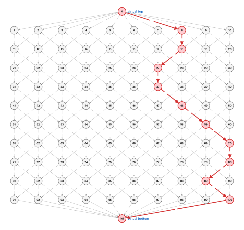
We observe that the graph structure isn’t actually necessary to store at all! Every graph for every image will have exactly the same structure as shown above, albeit with a different number of rows and columns.
A better approach than storing the graph structure is to operate directly on a 2D array of energies, i.e. effectively representing the graph with a 2D array of doubles, where the edges representing the structure of the graph are known implicitly. This is similar to what we did with heaps,
where we represented a PQ with an array of values corresponding to priorities, and the edges were known implicitly (e.g. that parent(k) = k/2).
Let’s explore this idea more carefully.
Part 5: Understanding the Greedy Shortest Paths Algorithm
Above, we saw that simply picking the cheapest pixel does not give the best result. However, if we’re clever, there is a greedy algorithm that does work and avoids any need to create an explicit Graph object.
Note: The idea use here will be covered in CS 170 and is called “Dynamic Programming”. You don’t need to know what this term means in 61B.
The core idea is that you start by computing a shortest paths matrix M row by row from top to
bottom, then walk back up the shortest paths matrix.
Suppose we have the following definitions:
- $M(i, j)$ - total cost of shortest cost path ending at (i, j)
- $e(i, j)$ - energy of pixel at location (i, j)
The top row is trivial, $M(i, 0)$ is just $e(i, 0)$ for all $i$. For lower rows, we can find $M(i, j)$ simply by adding the $e(i, j)$ to the minimum cost path ending at its top left, top middle, and top right pixels, or more formally:
$M(i, j) = e(i, j) + min(M(i - 1, j - 1), M(i, j - 1), M(i + 1, j - 1))$
Let’s watch this happen on the same 10-by-10 picture from Part 4. On the left is its energy matrix $E$, exactly the numbers you worked with by hand earlier. On the right we’ll build $M$, where $M(i, j)$ is the cost of the shortest path from the top row that ends at pixel $(i, j)$.
Click Compute M. The top row of $M$ appears first, since $M(i, 0) = e(i, 0)$. Then click Next row repeatedly. Each click fills in one more row: every entry is its own energy plus the smallest of the (up to) three entries above it, and the animation shows which cells are being looked at. Once the whole table is done, follow the instructions under it to read the seam off of $M$.
Part 6: computeM() and findSeamFromM()
Open SeamCarver.java. Here is its API.
You’ll write two methods: computeM computes $M$ from top to bottom. Then
findSeamFromM walks back up $M$ to get the seam.
Everything else is fully written.
public class SeamCarver {
    public SeamCarver(Picture picture)
    public Picture picture()                       // current picture
    public     int width()                         // width of current picture
    public     int height()                        // height of current picture
    public  double energy(int x, int y)            // energy of pixel at column x and row y

    public static double[][] computeM(double[][] energy)   // the M table for an energy table  <-- YOU WRITE THIS
    public static    int[] findSeamFromM(double[][] m)    // the seam encoded by an M table    <-- YOU WRITE THIS

    public   int[] findVerticalSeam()              // = findSeamFromM(computeM(energy))
    public   int[] findHorizontalSeam()            // sequence of indices for horizontal seam
    public    void removeHorizontalSeam(int[] seam)   // remove horizontal seam from picture
    public    void removeVerticalSeam(int[] seam)     // remove vertical seam from picture
}
More details:
computeM(double[][] e) returns a table of the same size as e. Fill
it in one row at a time, top to bottom, with loops (not recursion).
findSeamFromM(double[][] m) returns an array of length height such
that entry y is the column of the seam’s pixel in row y. For example, for the
10-by-10 shortest paths matrix $M$ above, you’d return
[7, 7, 6, 6, 7, 8, 9, 9, 8, 9].
All matrices are indexed [x][y], e.g. e[x][y] is
the energy of the pixel in column x and row y, so e.length is the width and
e[0].length is the height.
When there are multiple vertical seams with minimal total energy, your method can return any such seam.
Implement computeM, and run testComputeMOnSpecGrid to check it against
the table from Part 5. Then implement findSeamFromM, and run
testFindSeamFromMOnSpecGrid, which hands your method the correct $M$ for
that grid, so it passes or fails on its own regardless of your computeM.
When both pass, every test in SeamCarverTest should pass, including
testAllReferenceImages, which runs your code on every image in images/
and compares against the reference files. You can also run PrintSeams on
any small image and compare to its .printseams.txt file.
Then run SeamCarverVisualizer again (stop the old one first), load a photo,
and click GO. Each red line you see is exactly the seam your two methods
produced, drawn over the picture just before it is removed. A correct seam
looks a bit like lightning. As the animation runs, these lightning strikes should
wind their way through the flattest, most boring parts of the photo, shrinking
the image as it goes.
What about horizontal seams?
findHorizontalSeam is provided. It transposes the energy table (so that
rows become columns), runs your computeM and findSeamFromM on the
transposed table, and hands back the result, which is already indexed by
column and holds row numbers, exactly what a horizontal seam is. Have a look at it: the idea that
you can solve a new problem by reshaping it into one you’ve already solved
could easily appear on the final exam. The visualizer alternates between
vertical and horizontal seams so that both dimensions of your picture finish
shrinking together.
Checkoff
As you work through the lab, check in with your TA as a group to get attendance credit. Your TA will explain how check-ins work in your section.
For your checkoff, drop a photo of your choosing into the visualizer, shrink it, and show your TA. Then, be prepared to answer a few questions about your visualizer.
If you are not done coding, this is totally ok! As long as you have done Parts 1-5, you can answer the checkoff questions.
You do not need to have everything 100% correct to get credit. Keep working on the lab while you wait for your TA!
Extra Fun
Try out your SeamCarver on various real world images. Human or animal faces
are interesting as you see the algorithm try its best not to mess up the face before
eventually running out of low energy seams.
Deliverables
There is nothing to submit. Complete findVerticalSeam and get checked off by
your TA during lab.
Credits
This assignment was originally developed by Josh Hug, with supporting development work by Maia Ginsburg and Kevin Wayne at Princeton University.